Packages
library(raster)
library(rJava)
library(OpenStreetMap)
library(RgoogleMaps)
library(grid)
library(rgdal)
library(tidyverse)
library(reshape2)
library(ggmosaic)
library(GISTools)
library(sp)
library(sf)
library(tmap)
library(tmaptools)
library(mapview)
# carregar o dado
data("georgia")
# converter o dado em sf
georgia_sf <- st_as_sf(georgia)
class(georgia_sf)## [1] "sf" "data.frame"georgia_sf # representa as dez primeiras feições## Simple feature collection with 159 features and 14 fields
## Geometry type: MULTIPOLYGON
## Dimension: XY
## Bounding box: xmin: -85.6052 ymin: 30.35541 xmax: -80.84126 ymax: 35.00068
## CRS: +proj=longlat +ellps=WGS84
## First 10 features:
## Latitude Longitud TotPop90 PctRural PctBach PctEld PctFB PctPov PctBlack
## 0 31.75339 -82.28558 15744 75.6 8.2 11.43 0.64 19.9 20.76
## 1 31.29486 -82.87474 6213 100.0 6.4 11.77 1.58 26.0 26.86
## 2 31.55678 -82.45115 9566 61.7 6.6 11.11 0.27 24.1 15.42
## 3 31.33084 -84.45401 3615 100.0 9.4 13.17 0.11 24.8 51.67
## 4 33.07193 -83.25085 39530 42.7 13.3 8.64 1.43 17.5 42.39
## 5 34.35270 -83.50054 10308 100.0 6.4 11.37 0.34 15.1 3.49
## 6 33.99347 -83.71181 29721 64.6 9.2 10.63 0.92 14.7 11.44
## 7 34.23840 -84.83918 55911 75.2 9.0 9.66 0.82 10.7 9.21
## 8 31.75940 -83.21976 16245 47.0 7.6 12.81 0.33 22.0 31.33
## 9 31.27424 -83.23179 14153 66.2 7.5 11.98 1.19 19.3 11.62
## X Y ID Name MedInc geometry
## 0 941396.6 3521764 13001 Appling 32152 MULTIPOLYGON (((-82.2252 31...
## 1 895553.0 3471916 13003 Atkinson 27657 MULTIPOLYGON (((-82.6293 31...
## 2 930946.4 3502787 13005 Bacon 29342 MULTIPOLYGON (((-82.52171 3...
## 3 745398.6 3474765 13007 Baker 29610 MULTIPOLYGON (((-84.1407 31...
## 4 849431.3 3665553 13009 Baldwin 36414 MULTIPOLYGON (((-83.27423 3...
## 5 819317.3 3807616 13011 Banks 41783 MULTIPOLYGON (((-83.39851 3...
## 6 803747.1 3769623 13013 Barrow 49829 MULTIPOLYGON (((-83.53751 3...
## 7 699011.5 3793408 13015 Bartow 47309 MULTIPOLYGON (((-84.6533 34...
## 8 863020.8 3520432 13017 Ben Hill 28009 MULTIPOLYGON (((-83.17781 3...
## 9 859915.8 3466377 13019 Berrien 33786 MULTIPOLYGON (((-83.1461 31...Uma introdução ao package tmap
O package tmap permite o uso de novas funcionalidades para gerar mapas e funções para extração de dados do Google Maps e do OpenStreetMap. O foco do package tmap é a construção de mapas temáticos. Podem ser considerados dados sp e sf. A gramática para construção dos mapas é similar àquela do package ggplot. Assim, a representação de dados espaciais por meio do tmap conta com a manipulação de cada elemento do mapa separadamente em diferentes camadas.
Para limpar o workspace, digite:
rm(list=ls())Quick tmap
A função qtm() pode ser utilizada para composição de mapas de maneira expressa (quick). O código a seguir permite carregar o dado georgia, recriar o dado georgia_sf e gerar um mapa expresso.
data("georgia")
ls()
## [1] "georgia" "georgia.polys" "georgia2"Para criar o objeto sf georgia_sf, faça:
georgia_sf <- st_as_sf(georgia)Finalmente, crie o mapa expresso utilizando:
library(tmap)
qtm(georgia, fill="red", style = "natural")
O uso do parâmetro style permite configurações rápidas de mapas por meio do package tmap. Explore a função qtm para entender os demais temas possíveis.
O parâmetro fill pode ser utilizado para especificar uma cor ou a variável a ser mapeada.
qtm(georgia_sf, fill = "MedInc", text ="Name", text.size=0.5, format = "World_wide", style = "classic", text.root = 5, fill.title = "Median Income")
Mapa completo por meio do tmap
Para gerar mapas completos por meio do package tmap, é necessário utilizar a função tm_shapeacompanhada de uma outra função que especifique o precisa ser plotado. Antes de plotar, um objeto contendo a linha da divisa estadual da Georgia pode ser criada por meio da função st_union() do package sf. Uma alternativa para dados sp é função gUnaryUnion() do package rgeos, carregado juntamente com o package GISTools.
# união das feições para composição do limite estadual
g <- st_union(georgia_sf)

# plotar as camadas espaciais
tm_shape(georgia_sf) +
  tm_fill("tomato") +
  tm_borders(lty="dashed", col = "gold")
Incluir alguns estilos:
# plotar as camadas espaciais
tm_shape(georgia_sf) +
  tm_fill("tomato") +
  tm_borders(lty="dashed", col = "gold") +
  tm_style("natural", bg.color = "grey90")
Incluir limite estadual. Repare que a função tm_shape vai ser chamada novamente uma vez que outro objeto será incluído no mapa.
tm_shape(georgia_sf) +
  tm_fill("tomato") +
  tm_borders(lty="dashed", col = "gold") +
  tm_style("natural", bg.color = "grey90") +
  tm_shape(g) +
  tm_borders(lwd=2) # lwd - line width - espessura da linha
Incluindo todos os parâmetros juntos:
tm_shape(georgia_sf) +
  tm_fill("tomato") +
  tm_borders(lty="dashed", col = "gold") +
  tm_style("natural", bg.color = "grey90") +
  tm_shape(g) +
  tm_borders(lwd=2) +
  tm_layout(title = "O estado da Georgia",
            title.size = 1,
            title.position = c(0.55, "top"))
Experimente esses outros parâmetros da função qtm.
data(World, rivers, metro, land)

# just the map
qtm(World)
# choropleth
qtm(World, fill = "economy", format = "World", style = "col_blind")
# choropleth with more specifications
qtm(World, fill="HPI", fill.n = 9, fill.palette = "div",
    fill.title = "Happy Planet Index", fill.id = "name",
    style = "gray", format = "World")
# Alternative to previous map - RECOMENDED
tm_shape(World) +
    tm_polygons("HPI", n = 9, palette = "div",
        title = "Happy Planet Index", id = "name") +
    tm_style("gray") +
    tm_format("World")
# Bubble map
qtm(World, borders = NULL) +
qtm(metro, symbols.size = "pop2010",
    symbols.title.size= "Metropolitan Areas",
    symbols.id= "name",
    format = "World")
Para plotar dois mapas juntos com dados diferentes, experimente o seguinte código:
library(tmap)

t1 <- tm_shape(georgia_sf) +
              tm_fill("coral") +
              tm_borders() +
              tm_layout(bg.color = "grey85")

t2 <- tm_shape(georgia2) +
              tm_fill("orange") +
              tm_borders() +
              tm_layout(asp=0.86, bg.color = "grey95") #alinhar a segunda figura
t1
t2
Para especificar o layout da figura combinando os mapas:
library(grid)

# abrir uma nova página de plotagem
grid.newpage()

# definir o layout
pushViewport(viewport(layout = grid.layout(1,2)))

#  Plotar usando o comando print
print(t1, vp=viewport(layout.pos.col = 1, height = 5))
print(t2, vp=viewport(layout.pos.col = 2, height = 5))
Repare que t1 é um objeto
 sf e t2 é um objeto sp e apresentam sistemas de referência diferentes.
Para consultar os diferentes sistemas de projeção, verifique utilizando a função crs.
crs(georgia_sf)## CRS arguments: +proj=longlat +ellps=WGS84 +no_defscrs(georgia2)## CRS arguments:
## +proj=aea +lat_1=29.5 +lat_2=45.5 +lat_0=23 +lon_0=-96 +x_0=0.0
## +y_0=0.0 +ellps=GRS80 +units=m +datum=NAD83 +no_defs +towgs84=0,0,0Para nomear os atributos, verifique o data.frame do objeto georgia_sf. Utilize a função names() para ter acesso a uma lista de nomes de todos os atributos.
names(georgia_sf)## [1] "Latitude" "Longitud" "TotPop90" "PctRural" "PctBach" "PctEld"
## [7] "PctFB" "PctPov" "PctBlack" "X" "Y" "ID"
## [13] "Name" "MedInc" "geometry"# Construir um data frame com os nomes.
data.frame(georgia_sf)[,13]## [1] "Appling" "Atkinson" "Bacon" "Baker"
## [5] "Baldwin" "Banks" "Barrow" "Bartow"
## [9] "Ben Hill" "Berrien" "Bibb" "Bleckley"
## [13] "Brantley" "Brooks" "Bryan" "Bulloch"
## [17] "Burke" "Butts" "Calhoun" "Camden"
## [21] "Candler" "Carroll" "Catoosa" "Charlton"
## [25] "Chatham" "Chattahoochee" "Chattooga" "Cherokee"
## [29] "Clarke" "Clay" "Clayton" "Clinch"
## [33] "Cobb" "Coffee" "Colquitt" "Columbia"
## [37] "Cook" "Coweta" "Crawford" "Crisp"
## [41] "Dade" "Dawson" "Decatur" "DeKalb"
## [45] "Dodge" "Dooly" "Dougherty" "Douglas"
## [49] "Early" "Echols" "Effingham" "Elbert"
## [53] "Emanuel" "Evans" "Fannin" "Fayette"
## [57] "Floyd" "Forsyth" "Franklin" "Fulton"
## [61] "Gilmer" "Glascock" "Glynn" "Gordon"
## [65] "Grady" "Greene" "Gwinnett" "Habersham"
## [69] "Hall" "Hancock" "Haralson" "Harris"
## [73] "Hart" "Heard" "Henry" "Houston"
## [77] "Irwin" "Jackson" "Jasper" "Jeff Davis"
## [81] "Jefferson" "Jenkins" "Johnson" "Jones"
## [85] "Lamar" "Lanier" "Laurens" "Lee"
## [89] "Liberty" "Lincoln" "Long" "Lowndes"
## [93] "Lumpkin" "McDuffie" "McIntosh" "Macon"
## [97] "Madison" "Marion" "Meriwether" "Miller"
## [101] "Mitchell" "Monroe" "Montgomery" "Morgan"
## [105] "Murray" "Muscogee" "Newton" "Oconee"
## [109] "Oglethorpe" "Paulding" "Peach" "Pickens"
## [113] "Pierce" "Pike" "Polk" "Pulaski"
## [117] "Putnam" "Quitman" "Rabun" "Randolph"
## [121] "Richmond" "Rockdale" "Schley" "Screven"
## [125] "Seminole" "Spalding" "Stephens" "Stewart"
## [129] "Sumter" "Talbot" "Taliaferro" "Tattnall"
## [133] "Taylor" "Telfair" "Terrell" "Thomas"
## [137] "Tift" "Toombs" "Towns" "Treutlen"
## [141] "Troup" "Turner" "Twiggs" "Union"
## [145] "Upson" "Walker" "Walton" "Ware"
## [149] "Warren" "Washington" "Wayne" "Webster"
## [153] "Wheeler" "White" "Whitfield" "Wilcox"
## [157] "Wilkes" "Wilkinson" "Worth"Para incluir os nomes, faça:
tm_shape(georgia_sf) +
              tm_fill("white") +
              tm_borders() +
              tm_text("Name", size=0.3) +
              tm_layout(frame = FALSE)
Para criar um subconjunto dos dados, é possível fazer uma seleção criando uma camada com o subconjunto por meio dos índices:
index <- c(81, 82, 83, 150, 62, 53, 21, 16, 124, 121, 17)
georgia_sub <- georgia_sf[index, ]
Para sobrepor os mapas com as duas camadas, faça:
tm_shape(georgia_sf) +
              tm_fill("white") +
              tm_borders("grey", lwd=0.5) +
tm_shape(g) +
              tm_borders(lwd=2) +
tm_shape(georgia_sub) +
              tm_fill("lightblue") +
              tm_borders() +
              tm_layout(frame = TRUE, title = "Georgia com subconjunto", title.size=1, title.position = c(0.02, "bottom"))
Sistemas de coordenadas
Verificar qual o sistema de referência em uso de dados espaciais vetoriais
library(sf)
st_crs(georgia_sf)
## Coordinate Reference System:
## User input: +proj=longlat +ellps=WGS84
## wkt:
## GEOGCRS["unknown",
## DATUM["Unknown based on WGS84 ellipsoid",
## ELLIPSOID["WGS 84",6378137,298.257223563,
## LENGTHUNIT["metre",1],
## ID["EPSG",7030]]],
## PRIMEM["Greenwich",0,
## ANGLEUNIT["degree",0.0174532925199433],
## ID["EPSG",8901]],
## CS[ellipsoidal,2],
## AXIS["longitude",east,
## ORDER[1],
## ANGLEUNIT["degree",0.0174532925199433,
## ID["EPSG",9122]]],
## AXIS["latitude",north,
## ORDER[2],
## ANGLEUNIT["degree",0.0174532925199433,
## ID["EPSG",9122]]]]Verificar qual o sistema de referência em uso em dados espaciais matriciais
library(raster)
# crs(elev.r)
Sintaxe Proj4
| Parâmetro | Significado |
|---|---|
| +a | Semimajor radius of the ellipsoid axis |
| +b | Semiminor radius of the ellipsoid axis |
| +datum | Datum name |
| +ellps | Ellipsoid name |
| +lat_0 | Latitude of origin |
| +lat_1 | Latitude of first standard parallel |
| +lat_2 | Latitude of second standard parallel |
| +lat_ts | Latitude of true scale |
| +lon_0 | Central meridian |
| +over | Allow longitude output outside -180 to 180 range, disables wrapping |
| +proj | Projection name |
| +south | Denotes southern hemisphere UTM zone |
| +units | meters, US survey feet, etc. |
| +x_0 | False easting |
| +y_0 | False northing |
| +zone | UTM zone |
Base de dados EPGS
Alterar projeções
georgia_sf_crs <- st_transform(georgia_sf, crs = 3035)

st_crs(georgia_sf_crs)
Como salvar meu mapa
data(newhaven)

pdf(file = 'map.pdf') # salva o mapa como pdf.

tm_shape(blocks) +
    tm_borders() +
tm_shape(roads) +
  tm_lines(col = "red") +
# embellish the map
tm_scale_bar(width = 0.22) +
tm_compass(position = c(0.8, 0.07)) +
tm_layout(frame = F, title = "New Haven, CT",
            title.size = 1.5,
            title.position = c(0.55, "top"),
            legend.outside = T)

dev.off() # desconectar o arquivo gerado do ambiente de trabalho.
É possível salvar por meio de outros formatos.
pdf()
png()
tiff()
Adicionando mapa de contexto
Em algumas situações um mapa de fundo é interessante. Há várias maneiras de fazer essa inclusão. Pelo OpenStreetMap, a ideia é fazer a definição da área a ser representada, fazer o download e plotar o mapa de fundo. Depois acrescentar o mapa em desenvolvimento.
library(OpenStreetMap)
# define upper left, lower right corners
georgia.sub <- georgia[index,]
ul <- as.vector(cbind(bbox(georgia.sub)[2,2],
    bbox(georgia.sub)[1,1]))
lr <- as.vector(cbind(bbox(georgia.sub)[2,1],
    bbox(georgia.sub)[1,2]))
# download the map tile
MyMap <- openmap(ul,lr)
# now plot the layer and the backdrop
par(mar = c(0,0,0,0))
plot(MyMap, removeMargin=FALSE)
plot(spTransform(georgia.sub, osm()), add = TRUE, lwd = 2)
Visualização de fenômenos sociais no espaço
Mapas coropléticos
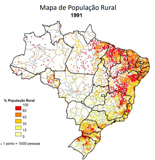
Mapas de pontos
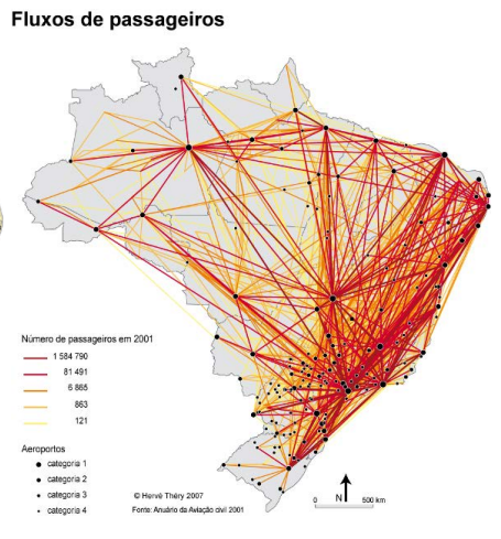
Representação de fluxos
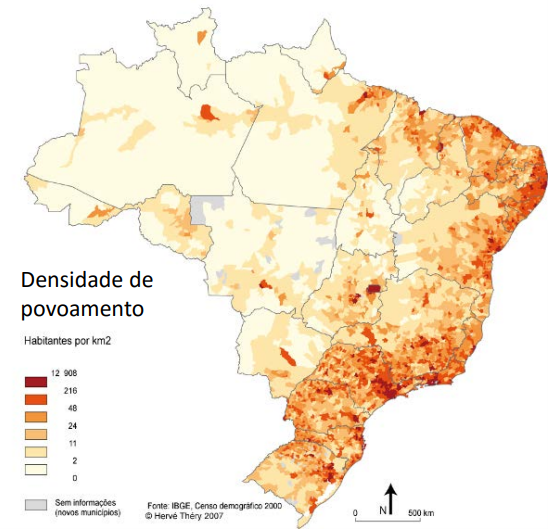
Mapas de calor

Cartogramas
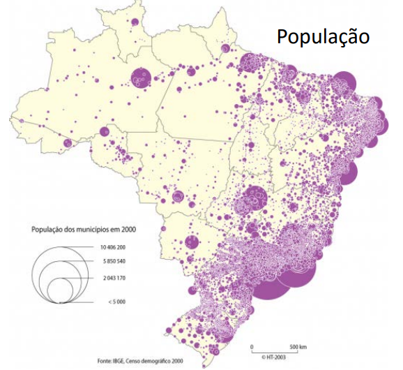
Símbolos proporcionais